
Differential and Integral Calculus 2021
1. Sequences
Chapter 1:
- Basics of sequences
- Some important sequences
- Convergence, divergence and limits
Basics of sequences
This section contains the most important definitions about sequences. Through these definitions the general notion of sequences will be explained, but then restricted to real number sequences.
Definition: Sequence
Let \(M\) be a non-empty set. A sequence is a function:
\[f:\mathbb{N}\rightarrow M.\]
Occasionally we speak about a sequence in \(M\).
Note. Characteristics of the set \(\mathbb{N}\) give certain characteristics to the sequence. Because \(\mathbb{N}\) is ordered, the terms of the sequence are ordered.
Definition: Terms and Indices
A sequence can be denoted denoted as
\((a_{1}, a_{2}, a_{3}, \ldots) = (a_{n})_{n\in\mathbb{N}} = (a_{n})_{n=1}^{\infty} = (a_{n})_{n}\)
instead of \(f(n).\) The numbers \(a_{1},a_{2},a_{3},\ldots\in M\) are called the terms of the sequence.
Because of the mapping \[\begin{aligned} f:\mathbb{N} \rightarrow & M \\ n \mapsto & a_{n}\end{aligned}\] we can assign a unique number \(n\in\mathbb{N}\) to each term. We write this number as a subscript and define it as the index; it follows that we can identify any term of the sequence by its index.
| n | 1 | 2 | 3 | 4 | 5 | 6 | 7 | 8 | 9 | \(\ldots\) |
|---|---|---|---|---|---|---|---|---|---|---|
| \(\downarrow\) | \(\downarrow\) | \(\downarrow\) | \(\downarrow\) | \(\downarrow\) | \(\downarrow\) | \(\downarrow\) | \(\downarrow\) | \(\downarrow\) | ||
| \(a_{n}\) | \(a_{1}\) | \(a_{2}\) | \(a_{3}\) | \(a_{4}\) | \(a_{5}\) | \(a_{6}\) | \(a_{7}\) | \(a_{8}\) | \(a_{9}\) | \(\ldots\) |
A few easy examples
Example 1: The sequence of natural numbers
The sequence \((a_{n})_{n}\) defined by \(a_{n}:=n,\,n\in \mathbb{N}\) is called the sequence of natural numbers. Its first few terms are: \[a_1=1,\, a_2=2,\, a_3=3, \ldots\] This special sequence has the property that every term is the same as its index.
![]()
Example 2: The sequence of triangular numbers
Triangular numbers get their name due to the following geometric visualization: Stacking coins to form a triangular shape gives the following diagram:
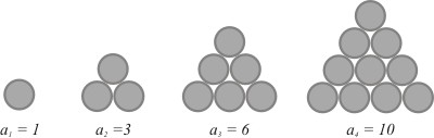
To the first coin in the first layer we add two coins in a second layer to form the second picture \(a_2\). In turn, adding three coins to \(a_2\) forms \(a_3\). From a mathematical point of view, this sequence is the result of summing natural numbers. To calculate the 10th triangular number we need to add the first 10 natural numbers: \[D_{10} = 1+2+3+\ldots+9+10\] In general form the sequence is defined as: \(D_{n} = 1+2+3+\ldots+(n-1)+n.\)
This motivates the following definition:
Notation and Definition: Sum sequence
Let \((a_n)_n, a_n: \mathbb{N}\to M\) be a sequence with terms \(a_n\), the sum is written: \[a_1 + a_2 + a_3 + \ldots + a_{n-1} + a_n =: \sum_{k=1}^n a_k\] The sign \(\sum\) is called sigma. Here, the index \(k\) increases from 1 to \(n\).
Sum sequences are sequences whose terms are formed by summation of previous terms.
Thus the nth triangular number can be written as: \[D_n = \sum_{k=1}^n k\]
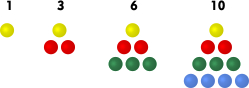
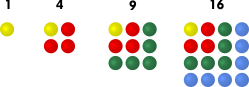
Example 3: Sequence of square numbers
The sequence of square numbers \((q_n)_n\) is defined by: \(q_n=n^2\). The terms of this sequence can also be illustrated by the addition of coins.
Interestingly, the sum of two consecutive triangular numbers is a square number. So, for example, we have: \(3+1=4\) and \(6+3=9\). In general this gives the relationship:
\[q_n=D_n + D_{n-1}\]
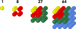
Example 4: Sequence of cube numbers
Analogously to the sequence of square number, we give the definition of cube numbers as \[a_n := n^3.\] The first terms of the sequence are: \((1,8,27,64,125,\ldots)\).
Example 5.
Let \((q_n)_n\) with \(q_n := n^2\) be the sequence of square numbers \[\begin{aligned}(1,4,9,16,25,36,49,64,81,100 \ldots)\end{aligned}\] and define the function \(\varphi(n) = 2n\). The composition \((q_{2n})_n\) yields: \[\begin{aligned}(q_{2n})_n &= (q_2,q_4,q_6,q_8,q_{10},\ldots) \\ &= (4,16,36,64,100,\ldots).\end{aligned}\]
Definition: Sequence of differences
Given a sequence \((a_{n})_{n}=a_{1},\, a_{2},\, a_{3},\ldots,\, a_{n},\ldots\); then \[(a_{n+1}-a_{n})_{n}:=a_{2}-a_{1}, a_{3}-a_{2},\dots\] is called the 1st difference sequence of \((a_{n})_{n}\)
The 1st difference sequence of the 1st difference sequence is called the 2nd difference sequence. Analogously the \(n\)th difference< sequence is defined.
Example 6.
Given the sequence \((a_n)_n\) with \(a_n := \frac{n^2+n}{2}\), i.e. \[\begin{aligned}(a_n)_n &= (1,3,6,10,15,21,28,36,\ldots)\end{aligned}\] Let \((b_n)_n\) be its 1st difference sequence. Then it follows that \[\begin{aligned}(b_n)_n &= (a_2-a_1, a_3-a_2, a_4-a_3,\ldots) \\ &= (2,3,4,5,6,7,8,9)\end{aligned}\] A term of \((b_n)_n\) has the general form \[\begin{aligned}b_n &= a_{n+1}-a_{n} \\ &= \frac{(n+1)^2+(n+1)}{2} - \frac{n^2+n)}{2} \\ &= \frac{(n+1)^2+(n+1)-n^2 - n }{2} \\ &= \frac{(n^2+2n+1)+1-n^2}{2} \\ &= \frac{2n+2}{2} \\ &= n + 1.\end{aligned}\]
Some important sequences
There are a number of sequences that can be regarded as the basis of many ideas in mathematics, but also can be used in other areas (e.g. physics, biology, or financial calculations) to model real situations. We will consider three of these sequences: the arithmetic sequence, the geometric sequence, and Fibonacci sequence, i.e. the sequence of Fibonacci numbers.
The arithmetic sequence
There are many definitions of the arithmetic sequence:
Definition A: Arithmetic sequence
A sequence \((a_{n})_{n}\) is called the arithmetic sequence, when the difference \(d \in \mathbb{R}\) between two consecutive terms is constant, thus: \[a_{n+1}-a_{n}=d \text{ with } d=const.\]
Note: The explicit rule of formation follows directly from definition A: \[a_{n}=a_{1}+(n-1)\cdot d\] For the \(n\)th term of an arithmetic sequence we also have the recursive formation rule: \[a_{n+1}=a_n + d.\]
Definition B: Arithmetic sequence
A non-constant sequence \((a_{n})_{n}\) is called an arithmetic sequence (1st order) when its 1st difference sequence is a sequence of constant value.
This rule of formation gives the arithmetic sequence its name: The middle term of any three consecutive terms is the arithmetic mean of the other two, for example:
\[a_2 = \frac{a_1+a_3}{2}.\]
Example 1.
The sequence of natural numbers \[(a_n)_n = (1,2,3,4,5,6,7,8,9,\ldots)\] is an arithmetic sequence, because the difference, \(d\), between two consecutive terms is always given as \(d=1\).
The geometric sequence
The geometric sequence has multiple definitions:
Definition: Geometric sequence
A sequence \((a_{n})_{n}\) is called a geometric sequence when the ratio of any two consecutive terms is always constant \(q\in\mathbb{R}\), thus \[\frac{a_{n+1}}{a_{n}}=q \text{ for all } n\in\mathbb{N}.\]
Note.The recursive relationship \(a_{n+1} = q\cdot a_n \) of the terms of the geometric sequence and the explicit formula for the calculation of the n th term of a geometric sequence \[a_n=a_1\cdot q^{n-1}\] follows directly from the definition.
Again the name and the rule of formation of this sequence are connected: Here, the middle term of three consecutive terms is the geometric mean of the other two, e.g.: \[a_2 = \sqrt{a_1\cdot a_3}.\]
Example 2.
Let \(a\) and \(q\) be fixed positive numbers. The sequence \((a_n)_n\) with \(a_n := aq^{n-1}\), i.e. \[\left( a_1, a_2, a_3, a_4,\ldots \right) = \left( a, aq, aq^2, aq^3,\ldots \right)\] is a geometric sequence. If \(q\geq1\) the sequence is monotonically increasing. If \(q<1\) it is strictly decreasing. The corresponding range \({a,aq,aq^2, aq^3}\) is finite in the case \(q=1\) (namely, a singleton), otherwise it is infinite.
The Fibonacci sequence
The Fibonacci sequence is famous because it plays a role in many biological processes, for instance in plant growth, and is frequently found in nature. The recursive definition is:
Definition: Fibonacci sequence
Let \(a_0 = a_1 = 1\) and let \[a_n := a_{n-2}+a_{n-1}\] for \(n\geq2\). The sequence \((a_n)_n\) is then called the Fibonacci sequence. The terms of the sequence are called the Fibonacci numbers.
The sequence is named after the Italian mathematician Leonardo of Pisa (ca. 1200 AD), also known as Fibonacci (son of Bonacci). He considered the size of a rabbit population and discovered the number sequence: \[(1,1,2,3,5,8,13,21,34,55,\ldots),\]
Example 3.
The structure of sunflower heads can be described by a system of two spirals, which radiate out symmetrically but contra rotating from the centre; there are 55 spirals which run clockwise and 34 which run counter-clockwise.
Pineapples behave very similarly. There we have 21 spirals running in one direction and 34 running in the other. Cauliflower, cacti, and fir cones are also constructed in this manner.

Convergence, divergence and limits
The following chapter deals with the convergence of sequences. We will first introduce the idea of zero sequences. After that we will define the concept of general convergence.
Preliminary remark: Absolute value in \(\mathbb{R}\)
The absolute value function \(x \mapsto |x|\) is fundamental in the study of convergence of real number sequences. Therefore we should summarise again some of the main characteristics of the absolute value function:
Definition: Absolute Value
For any given number \(x\in\mathbb{R}\) its absolute value \(|x|\) is defined by \[\begin{aligned}|x|:=\begin{cases}x & \text{for }x\geq0,\\ -x & \text{for }x<0.\end{cases}\end{aligned}\]
Graph of the absolute value function
Theorem: Calculation Rule for the Absolute Value
For \(x,y\in\mathbb{R}\) the following is always true:
\(|x|\geq0,\)
\(|x|=0\) if and only if \(x=0.\)
\(|x\cdot y|=|x|\cdot|y|\) (Multiplicativity)
\(|x+y|\leq|x|+|y|\) (Triangle Inequality)
Parts 1.-3. Results follow directly from the definition and by dividing it up into separate cases of the different signs of \(x\) and \(y\)
Part 4. Here we divide the triangle inequality into different cases.
Case 1.
First let \(x,y \geq 0\). Then it follows that \[\begin{aligned}|x+y|=x+y=|x|+|y|\end{aligned}\] and the desired inequality is shown.
Case 2.Next let \(x,y < 0\). Then: \[\begin{aligned}|x+y|=-(x+y)=(-x)+ (-y)=|x|+|y|\end{aligned}\]
Case 3.Finally we consider the case \(x\geq 0\) and \(y<0\). Here we have two subcases:
For \(x \geq -y\) we have \(x+y\geq 0\) and thus \(|x+y|=x+y\) from the definition of absolute value. Because \(y<0\) then \(y<-y\) and therefore also \(x+y < x-y\). Overall we have: \[\begin{aligned}|x+y| = x+y < x-y = |x|+|y|\end{aligned}\]
For \(x < -y\) then \(x+y<0\). We have \(|x+y|=-(x+y)=-x-y\). Because \(x\geq0\), we have \(-x < x\) and thus \(-x-y\leq x-y\). Overall we have: \[\begin{aligned}|x+y| = -x-y \leq x-y = |x|+|y|\end{aligned}\]
The case \(x<0\) and \(y\geq0\) we prove it analogously to the case 3, in which \(x\) and \(y\) are exchanged.
\(\square\)
Zero sequences
Definition: Zero sequence
A sequence \((a_{n})_{n}\) s called a zero sequence, if for every \(\varepsilon>0,\) there exists an index \(n_{0}\in\mathbb{N}\) such that \[|a_{n}| < \varepsilon\] for every \(n\geq n_{0},\, n\in\mathbb{N}\). In this case we also say that the sequence converges to zero.
Informally: We have a zero sequence, if the terms of the sequence with high enough indices are arbitrarily close to zero.
Example 1.
The sequence \((a_n)_n\) defined by \(a_{n}:=\frac{1}{n}\), i.e. \[\left(a_{1},a_{2},a_{3},a_{4},\ldots\right):=\left(\frac{1}{1},\frac{1}{2},\frac{1}{3},\frac{1}{4},\ldots\right)\] is called the harmonic sequence. Clearly, it is positive for all \(n\in\mathbb{N}\), however as \(n\) increases the absolute value of each term decreases getting closer and closer to zero.
Take for example \(\varepsilon := \frac{1}{5000}\), then choosing the index \(n_0 = 5000\), it follows that \(a_n<\frac{1}{5000}=\varepsilon\), for all \(n\geq n_0\).
The harmonic sequence converges to zero
Example 2.
Consider the sequence \[(a_n)_n \text{ where } a_n:=\frac{1}{\sqrt{n}}.\] Let \(\varepsilon := \frac{1}{1000}\).We then obtain the index \(n_0=1000000\) in this manner that for all terms \(a_n\) where \(n\geq n_0\) \(a_n < \frac{1}{1000}=\varepsilon\).
Note. To check whether a sequence is a zero sequence, you must choose an (arbitrary) \(\varepsilon \in \mathbb{R}\) where \(\varepsilon > 0\). Then search for a index \(n_0\), after which all terms \(n\) are smaller then said \(\varepsilon\).
Example 3.
We consider the sequence \((a_n)_n\), defined by \[a_n := \left( -1 \right)^n \cdot \frac{1}{n^2}.\]
Because of the factors \((-1)^n\) two consecutive terms have different signs; we call a sequence whose signs change in this way an alternating sequence.
We want to show that this sequence is a zero sequence. According to the definition we have to show that for every \(\varepsilon > 0\) there exist \(n_0 \in \mathbb{N}\), such that we have the inequality: \[|a_n|< \varepsilon\] for every term \(a_n\) where \(n\geq n_0\).
Firstly we let \(\varepsilon > 0\) be an arbitrary constant. Because the inequality \( |a_n|< \varepsilon\) must hold true for an arbitrary \(\varepsilon\) we must find the index \(n_0\) which depends on each \(\varepsilon\). More exactly: The inequality \[|a_{n_0}|=\left| \frac{1}{{n_0}^2} \right|= \frac{1}{{n_0}^2}<\varepsilon\] must be true for the index \(n_0\). Solve for \(n_0\): \[n_0 > \frac{1}{\sqrt{\varepsilon}},\] this index \(n_0\) gives our desired characteristic for every \(\varepsilon\).
Negative examples
The following are examples of non-convergent alternating sequences:
\(a_n = (-1)^n\)
\(a_n = (-1)^n \cdot n\)
Theorem: Characteristics of Zero sequences
Let \((a_n)_n\) and \((b_n)_n\) be two sequences. Then:
Let \((a_n)_n\) be a zero sequence, if \(b_n = a_n\) or \(b_n = -a_n\) for all \(n\in\mathbb{N}\) then \((b_n)_n\) is also a zero sequence.
Let \((a_n)_n\) be a zero sequence, if \(-a_n\leq b_n \leq a_n\) for all \(n\in\mathbb{N}\) then \((b_n)_n\) is also a zero sequence.
Let \((a_n)_n\) be a zero sequence, then \((c\cdot a_n)_n\) where \(c \in \mathbb{R}\) is also a zero sequence.
If \((a_n)_n\) and \((b_n)_n\) are zero sequences, then \((a_n + b_n)_n\) is also a zero sequence.
Parts 1 and 2. If \((a_n)_n\) is a zero sequence, then according to the definition there is an index \(n_0 \in \mathbb{N}\), such that \(|a_n|<\varepsilon\) for every \(n\geq n_0\) and an arbitrary \(\varepsilon\in\mathbb{R}\). But then we have \(|b_n|\leq|a_n|<\varepsilon\); this proves parts 1 and 2 are correct.
Part 3. If \(c=0\), then the result is trivial. Let \(c\neq0\) and choose \(\varepsilon > 0\) such that \[\begin{aligned}|a_n|<\frac{\varepsilon}{|c|}\end{aligned}\] for all \(n\geq n_0\). Rearranging we get: \[\begin{aligned} |c|\cdot|a_n|=|c\cdot a_n|<\varepsilon\end{aligned}\]
Part 4.
Because \((a_n)_n\) is a zero sequence, by the definition we have \(|a_n|<\frac{\varepsilon}{2}\) for all \(n\geq n_0\). Analogously, for the zero sequence \((b_n)_n\) there is a \(m_0 \in \mathbb{N}\) with \(|b_n|<\frac{\varepsilon}{2}\) for all \(n\geq m_0\).
Then for all \(n > \max(n_0,m_0)\) it follows (using the triangle inequality) that: \[\begin{aligned}|a_n + b_n|\leq|a_n|+|b_n|<\frac{\varepsilon}{2}+\frac{\varepsilon}{2} = \varepsilon\end{aligned}\]
\(\square\)
Convergence, divergence
The concept of zero sequences can be expanded to give us the convergence of general sequences:
Definition: Convergence and Divergence
A sequence \((a_{n})_{n}\) is called convergent to \(a\in\mathbb{R}\), if for every \(\varepsilon>0\) there exists a \(n_{0}\) such that: \[|a_{n}-a| \lt \varepsilon \text{ for all }n\in\mathbb{N}_{0},\text{ where }n\geq n_{0}\]
An equivalent definition can be defined by:
A sequence \((a_{n})_{n}\) is called convergent to \(a\in\mathbb{R}\), if \((a_{n}-a)_{n}\) is a zero sequence.
Example 4.
We consider the sequence \((a_n)_n\) where \[a_n=\frac{2n^2+1}{n^2+1}.\] By plugging in large values of \(n\), we can see that for \(n\to\infty\) \(a_n \to 2\) and therefore we can postulate that the limit is \(a=2\).
To show this, we show that for every \(\varepsilon > 0\) there exists an index \(n_0\in\mathbb{N}\), such that for every term \(a_n\) with \(n>n_0\) the following relationship holds: \[\left| \frac{2n^2+1}{n^2+1} - 2\right| < \varepsilon.\]
Firstly we estimate the inequality: \[\begin{aligned}\left|\frac{2n^2+1}{n^2+1}-2\right| =&\left|\frac{2n^2+1-2\cdot\left(n^2+1\right)}{n^2+1}\right| \\ =&\left|\frac{2n^2+1-2n^2-2}{n^2+1}\right| \\ =&\left|-\frac{1}{n^2+1}\right| \\ =&\left|\frac{1}{n^2+1}\right| \\ <&\frac{1}{n},\end{aligned}\] The last step uses a crude approximation.
We let \(\varepsilon > 0\) be an arbitrary constant. Then we choose the index \(n_0\in\mathbb{N}\), such that \[n_0 > \frac{1}{\varepsilon} \text{, or equivalently, } \frac{1}{n_0} < \varepsilon.\] Finally from the above inequality we have: \[\left|\frac{2n^2+1}{n^2+1}-2\right| < \frac{1}{n} < \frac{1}{n_0} < \varepsilon,\] Thus we have proved the note above. Therefore \(a=2\) is the limit of the sequence.
\(\square\)
If a sequence is convergent, then there is exactly one number which is the limit. This characteristic is called the uniqueness of convergence.
Theorem: Uniqueness of Convergence
Let \((a_{n})_{n}\) be a sequence that converges to \(a\in\mathbb{R}\) and to \(b\in\mathbb{R}\). This implies \(a=b\).
Assume \(a\ne b\); choose \(\varepsilon\in\mathbb{R}\) with \(\varepsilon:=\frac{1}{3}|a-b|.\) Then in particular \([a-\varepsilon,a+\varepsilon]\cap[b-\varepsilon,b+\varepsilon]=\emptyset.\)
Because \((a_{n})_{n}\) converges to \(a\), there is, according to the definition of convergence, a index \(n_{0}\in\mathbb{N}\) with \(|a_{n}-a|< \varepsilon\) for \(n\geq n_{0}.\) Furthermore, because \((a_{n})_{n}\) converges to \(b\) there is also a \(\widetilde{n_{0}}\in\mathbb{N}\) with \(|a_{n}-b|< \varepsilon\) for \(n\geq\widetilde{n_{0}}.\) For \(n\geq\max\{n_{0},\widetilde{n_{0}}\}\) we have:
\[\begin{aligned}\varepsilon\ = &\ \frac{1}{3}|a-b| \Rightarrow\\
3\varepsilon\ = &\ |a-b|\\
= &\ |(a-a_{n})+(a_{n}-b)|\\
\leq &\ |a_{n}-a|+|a_{b}-b|\\
< &\ \varepsilon+\varepsilon=2\varepsilon,\end{aligned}\]
Consequently we have obtained \(3\varepsilon\leq2\varepsilon\), which is a contradiction as \(\varepsilon>0\). Therefore the assumption must be wrong, so \(a=b\).
\(\square\)
Definition: Divergent, Limit
If provided that a sequence \((a_{n})_{n}\) and an \(a\in\mathbb{R}\) exist, to which the sequence converges, then the sequence is called convergent and \(a\) is called the limit of the sequence, otherwise it is called divergent.
Notation. \((a_{n})_{n}\) is convergent to \(a\) is also written: \[a_{n}\rightarrow a,\text{ or }\lim_{n\rightarrow\infty}a_{n}=a.\] Such notation is allowed, as the limit of a sequence is always unique by the above Theorem (provided it exists).
Theorem: Bounded Sequences
A convergent sequence \((a_n)_n\) is bounded i.e. there exists a constant \(r\in\mathbb{R}\) such that: \[|a_n| \lt r\] for all \(n\in\mathbb{N}\).
We assume that the sequence \((a_n)_n\) has the limit \(a\). By the definition of convergence, we have that \(|a_n - a|<\varepsilon\) for all \(\varepsilon \in \mathbb{R}\) and \(n\geq n_0\). Choosing \(\varepsilon = 1\) gives:
\[\begin{aligned}|a_n|-|a|&\ \leq |a_n -a| \\
&\ < 1,\end{aligned}\]
And therefore also \(|a_n|\leq |a|+1\).
Thus for all \(n\in \mathbb{N}\): \[|a_n|\leq \max \left\{ |a_1|,|a_2|,\ldots,|a_{n_0}|,|a|+1 \right\}=:r\]
\(\square\)
Rules for convergent sequences
Theorem: Subsequences
Let \((a_{n})_{n}\) be a sequence such that \(a_{n}\rightarrow a\) and let \((a_{\varphi(n)})_{n}\) be a subsequence of \((a_{n})_{n}\). Then it follows that \((a_{\varphi(n)})_{n}\rightarrow a\).
Informally: If a sequence is convergent then all of its subsequences are also convergent and in fact converge to the same limit as the original.
By the definition of a subsequence \(\varphi(n)\geq n\). Because \(a_{n}\rightarrow a\) it is implicated that \(|a_{n}-a|<\varepsilon\) for \(n\geq n_{0}\), therefore \(|a_{\varphi(n)}-a|<\varepsilon\) for these indices \(n\).
\(\square\)
Theorem: Rules
Let \((a_{n})_{n}\) and \((b_{n})_{n}\) be sequences with \(a_{n}\rightarrow a\) and \(b_{n}\rightarrow b\). Then for \(\lambda, \mu \in \mathbb{R}\) it follows that:
\(\lambda \cdot (a_n)+\mu \cdot (b_n) \to \lambda \cdot a + \mu \cdot b\)
\((a_n)\cdot (b_n) \to a\cdot b\)
Informally: Sums, differences and products of convergent sequences are convergent.
Part 1. Let \(\varepsilon > 0\). We must show, that for all \(n \geq n_0\) it follows that: \[|\lambda \cdot a_n + \mu \cdot b_n - \lambda \cdot a - \mu \cdot b| < \varepsilon.\] The left hand side we estimate using: \[|\lambda (a_n-a)+\mu (b_n - b)| \leq |\lambda|\cdot|a_n-a|+|\mu|\cdot|b_n-b|.\]
Because \((a_n)_n\) and \((b_n)_n\) converge, for each given \(\varepsilon > 0\) it holds true that: \[\begin{aligned}|a_n - a| <\ \varepsilon_1 := &\ \textstyle \frac{\varepsilon}{2|\lambda|} \text{ for all }n\geq n_0\\ |b_n - b| <\ \varepsilon_2 := &\ \textstyle \frac{\varepsilon}{2|\mu|} \text{ for all }n\geq n_1\end{aligned}\]
Therefore \[\begin{aligned}|\lambda|\cdot|a_n-a|+|\mu|\cdot|b_n-b| < &\ |\lambda|\varepsilon_1 + |\mu|\varepsilon_2 \\ = &\ \textstyle{ \frac{\varepsilon}{2} + \frac{\varepsilon}{2} } = \varepsilon\end{aligned}\] for all numbers \(n \geq \max \{n_0,n_1\}\). Therefore the sequence \[\left( \lambda \left( a_n - a \right) + \mu \left( b_n - b \right) \right)_n\] is a zero sequence and the desired inequality is shown.
Part 2. Let \(\varepsilon > 0\). We have to show, that for all \(n > n_0\) \[|a_n b_n - a b| < \varepsilon.\] Furthermore an estimation of the left hand side follows: \[\begin{aligned} |a_n b_n - a b| =&\ |a_n b_n - a b_n + a b_n - ab| \\ \leq &\ |b_n|\cdot|a_n-a| + |a|\cdot|b_n - b|.\end{aligned}\] We choose a number \(B\), such that \(|b_n| \lt b\) for all \(n\) and \(|a| \lt b\). Such a value of \(B\) exists by the Theorem of convergent sequences being bounded. We can then use the estimation: \[\begin{aligned}|b_n|\cdot|a_n-a| + |a|\cdot|b_n - b| <&\ B \cdot \left(|a_n - a| + |b_n - b| \right).\end{aligned}\] For all \(n>n_0\) we have \(|a_n - a|<\frac{\varepsilon}{2\cdot B}\) and \(|b_n - b|<\frac{\varepsilon}{2\cdot B}\), and - putting everything together - the desired inequality it shown.
\(\square\)